Imagine you re-designing your e-commerce website. You have to decide
whether the "Buy Item" button should be blue or green. You decide to
setup an A/B test, so you build two versions of the item page:
- Page A which has a blue button;
- Page B which has a green button.
Pages A and B are identical except for the color of the button. You want
to quantify the likelihood of a user clicking the "Buy Item" button when
she is on page A or on page B. So, you start the experiment by sending
each user either to page A or to page B. Each time, you monitor whether
she clicked "Buy Item" or not.
Frequentist vs Bayesian
One could simply approximate the effectiveness of each page by computing
the success rate on the two pages. E.g. if N=1000 users visited page
A, and 50 of them clicked the button, one could say that the likelihood
of clicking the button on page A is 50/1000 \~= 5%. This is the
so-called Frequentist approach which envisions the probability in
terms of event frequency. However, the following issues might arise on a
daily basis:
- what if N is small (e.g. N=50)? Can we still be confident by just
computing the success rate?
- What if N is different between page A and page B? Let's say that 500
users visited page A and 2000 users visited page B. How can we
combine such imbalanced experiments?
- How large should N be to achieve a 90% confidence in my estimates?
We'll now introduce a simple Bayesian solution that allows to run
the A/B test and to handle the issues listed above. The code makes use
of PyMC package, and it was
inspired by reading "Bayesian Methods for Hackers" by Cameron
Davidson-Pilon.
Evaluate Page A
We'll first show how to evaluate the success rate on page A with a
Bayesian approach. The goal is to infer the probability of clicking the
"Buy Item" button on page A. We model this probability as a
Bernoulli
distribution with parameter \(p_A\):
$$P(click | \text{page}=A) =
\begin{cases}
p_A & click=1\\
1-p_A & click=0\\
\end{cases}$$
So, \(p_A\) is the parameter indicating the probability
of clicking the button on page A. This parameter is unknown and the goal
of the experiment is to infer it.
from pymc import Uniform, rbernoulli, Bernoulli, MCMC
from matplotlib import pyplot as plt
import numpy as np

# true value of p_A (unknown)
p_A_true = 0.05
# number of users visiting page A
N = 1500
occurrences = rbernoulli(p_A_true, N)

print 'Click-BUY:'
print occurrences.sum()
print 'Observed frequency:'
print occurrences.sum() / float(N)
In this code, we are simulating a realisation of the experiment where
1000 users visited page A. Here, occurrences indicate how many
visitors have actually clicked on the button in this realisation.
The next step consist of defining our prior on the
\(p_A\) parameter. The prior definition is the
first step of Bayesian inference and is a way to indicate our prior
belief in the variable.
p_A = Uniform('p_A', lower=0, upper=1)
obs = Bernoulli('obs', p_A, value=occurrences, observed=True)
In this section, we define the prior of \(p_a\) to be a
uniform distribution. The obs variable indicates the Bernoulli
distribution representing the observations of the click events (indeed
governed by the \(p_a\) parameter). The two variables
are assigned to Uniform and Bernoulli which are stochastic variable
objects part of PyMC. Each variable is associated with a string name
(p_A * and obs in this case). The obs variable has the value *
and the observed parameter set because we have observed the
realisations of the experiments.
# defining a Monte Carlo Markov Chain model
mcmc = MCMC([p_A, obs])
# setting the size of the simulations to 20k particles
mcmc.sample(20000, 1000)
# the resulting posterior distribution is stored in the trace variable
print mcmc.trace('p_A')[:]
In this section, the MCMC model is initialised, and the variables p_A
and obs are given to it as input. The sample model will run the
Monte Carlo simulations and fit the observed data to the prior belief.
The posterior distribution is accessible via the .trace attribute as
an array of realisations. We can now visualise the result of the
inference.
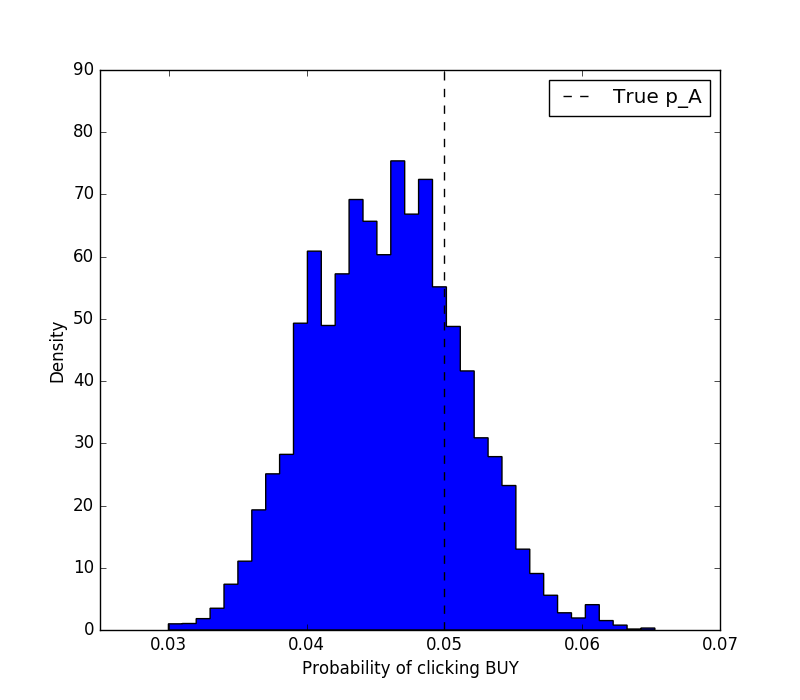
plt.figure(figsize=(8, 7))
plt.hist(mcmc.trace('p_A')[:], bins=35, histtype='stepfilled',
normed=True)
plt.xlabel('Probability of clicking BUY')
plt.ylabel('Density')
plt.vlines(p_A_true, 0, 90, linestyle='--', label='True p_A')
plt.legend()
plt.show()
 {.alignnone
.wp-image-38 .size-full width="800" height="700"}
{.alignnone
.wp-image-38 .size-full width="800" height="700"}
Then, we might want to answer the question: where am I 90% confident
that the true \(p_A\) lies? That's easy to answer.
p_A_samples = mcmc.trace('p_A')[:]
lower_bound = np.percentile(p_A_samples, 5)
upper_bound = np.percentile(p_A_samples, 95)
print 'There is 90%% probability that p_A is between %s and %s' %
(lower_bound, upper_bound)
# There is 90% probability that p_A is between 0.0373019596856 and
0.0548052806892
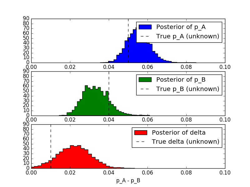
Comparing Page A and Page B
We'll now repeat what we have done for page A, and we add a new
variable delta indicating the difference
between \(p_A\) and \(p_B\).
from pymc import Uniform, rbernoulli, Bernoulli, MCMC, deterministic
from matplotlib import pyplot as plt

p_A_true = 0.05
p_B_true = 0.04
N_A = 1500
N_B = 750

occurrences_A = rbernoulli(p_A_true, N_A)
occurrences_B = rbernoulli(p_B_true, N_B)

print 'Observed frequency:'
print 'A'
print occurrences_A.sum() / float(N_A)
print 'B'
print occurrences_B.sum() / float(N_B)

p_A = Uniform('p_A', lower=0, upper=1)
p_B = Uniform('p_B', lower=0, upper=1)

@deterministic
def delta(p_A=p_A, p_B=p_B):
return p_A - p_B

obs_A = Bernoulli('obs_A', p_A, value=occurrences_A, observed=True)
obs_B = Bernoulli('obs_B', p_B, value=occurrences_B, observed=True)

mcmc = MCMC([p_A, p_B, obs_A, obs_B, delta])
mcmc.sample(25000, 5000)

p_A_samples = mcmc.trace('p_A')[:]
p_B_samples = mcmc.trace('p_B')[:]
delta_samples = mcmc.trace('delta')[:]

plt.subplot(3,1,1)
plt.xlim(0, 0.1)
plt.hist(p_A_samples, bins=35, histtype='stepfilled', normed=True,
color='blue', label='Posterior of p_A')
plt.vlines(p_A_true, 0, 90, linestyle='--', label='True p_A
(unknown)')
plt.xlabel('Probability of clicking BUY via A')
plt.legend()
plt.subplot(3,1,2)
plt.xlim(0, 0.1)
plt.hist(p_B_samples, bins=35, histtype='stepfilled', normed=True,
color='green', label='Posterior of p_B')
plt.vlines(p_B_true, 0, 90, linestyle='--', label='True p_B
(unknown)')
plt.xlabel('Probability of clicking BUY via B')
plt.legend()
plt.subplot(3,1,3)
plt.xlim(0, 0.1)
plt.hist(delta_samples, bins=35, histtype='stepfilled', normed=True,
color='red', label='Posterior of delta')
plt.vlines(p_A_true - p_B_true, 0, 90, linestyle='--', label='True
delta (unknown)')
plt.xlabel('p_A - p_B')
plt.legend()
plt.show()
 {.alignnone
.wp-image-40 .size-full width="800" height="600"}
{.alignnone
.wp-image-40 .size-full width="800" height="600"}
Then, we can answer a question like: what is the probability that
\( p_A > p_B\)?
print 'Probability that p_A > p_B:'
print (delta_samples > 0).mean()
# Probability that p_A > p_B
# 0.8919